The clever bin-sorting hack that correctly displays objects behind one another
One of the bigger challenges in 3D graphics is making sure that objects appear at the correct distances, and in particular that more distant objects are shown behind objects that are closer to the viewer. Nothing breaks immersion quite like a distant rocket overlapping a nearby tree, so it's vital that objects that are far away are drawn before objects that are closer, so the nearer objects can appear on top.
The issue is particularly relevant when we're flying low across the landscape, like this:
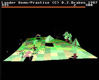
Not only do we want to make sure that the 3D objects are in the correct order, but we also need to make sure that all those particles appear at the right distance, otherwise things will just look like a mess. One approach is to sort everything by depth before drawing anything, and while this might work for the small number of objects on-screen at any one time, there are an awful lot of particles in Lander - up to 438 of them at any one time - and that's a lot of depth-sorting.
The problem is that sorting is an inherently slow process. There are plenty of clever sorting algorithms that optimise the process, but when you're building a fast-action game on a 1980s microcomputer, sorting isn't something you want to be doing on every iteration of the main loop.
Not surprisingly, David Braben found an elegant hack to get around the issue while still managing to keep Lander's objects and particles in order. The solution is called "bin-sorting", and that's what we're going to look at here.
The graphics buffers
--------------------
The bin-sorting solution does away with the need to sort anything. Instead, we define 11 graphics buffers (our "bins"), one for each row of tile corners on the landscape. The landscape is ten tiles deep, so there are 11 rows of tile corners, and we therefore have 11 graphics buffers.
Whenever we draw an object or a particle in the main game code, we don't actually draw anything onto the screen, but instead we put that item into the correct graphics buffer, according to how far away it is. If you imagine the buffers as a collection of big, dumpster-style bins, then when we draw an object, we look at the object's depth along the z-axis, and chuck it into the corresponding bin. We do the same with particles - into the bin they go. And then, when we've finished drawing everything, we can work our way through each bin, starting with the most distant bin and working our way forwards, drawing everything in a bin before moving on to the next one. Each graphics buffer is just a big bin that's full of objects and particles, all of which appear in the same tile row.
This approach doesn't require any sorting, and as long as it's a quick process to decide which graphics buffer we should be putting each object or particle into, then it's a scalable and efficient process. It isn't perfect, as items that appear in the same tile row are drawn in the order in which they were put into the buffer, so it is possible for objects to overlap incorrectly. In Lander, though, this isn't much of a problem, as objects are only placed on the map at tile corners, so all the ground-based objects in a buffer will be at exactly the same distance from the viewer anyway.
To be explicit, consider the landscape grid of tile corners that's described in the deep dive on drawing the landscape, where row a is the furthest from the viewer and row k is the closest:
     0    1    2    3    4    5    6    7    8    9   10   11   12

  a  +----+----+----+----+----+----+----+----+----+----+----+----+
     |    |    |    |    |    |    |    |    |    |    |    |    |
     |    |    |    |    |    |    |    |    |    |    |    |    |
  b  +----+----+----+----+----+----+----+----+----+----+----+----+
     |    |    |    |    |    |    |    |    |    |    |    |    |
     |    |    |    |    |    |    |    |    |    |    |    |    |
  c  +----+----+----+----+----+----+----+----+----+----+----+----+
     |    |    |    |    |    |    |    |    |    |    |    |    |
     :    :    :    :    :    :    :    :    :    :    :    :    :

     :    :    :    :    :    :    :    :    :    :    :    :    :
     |    |    |    |    |    |    |    |    |    |    |    |    |
  k  +----+----+----+----+----+----+----+----+----+----+----+----+
We define graphics buffer 0 as containing objects and particles in the first tile row, so that's any objects along corner row a, or on top of the tiles between rows a and b (but it doesn't contain any objects that are on corner row b).
Then we define graphics buffer 1 as containing objects and particles in the second tile row, so that's any objects on corner row b, or on top of the tiles between rows b and c (but not actually on corner row c).
This continues until we get to graphics buffer 10, which we define as all the objects and particles along corner row k, plus anything in front of the landscape (though see the next section for a bit more on this).
So the graphics buffers contain objects and particles according to their distance, like this:
     0    1    2    3    4    5    6    7    8    9   10   11   12

  a  +----+----+----+----+----+----+----+----+----+----+----+----+   Buffer 0
     |    |    |    |    |    |    |    |    |    |    |    |    |      |
     |    |    |    |    |    |    |    |    |    |    |    |    |      v
  b  +----+----+----+----+----+----+----+----+----+----+----+----+   Buffer 1
     |    |    |    |    |    |    |    |    |    |    |    |    |      |
     |    |    |    |    |    |    |    |    |    |    |    |    |      v
  c  +----+----+----+----+----+----+----+----+----+----+----+----+   Buffer 2
     |    |    |    |    |    |    |    |    |    |    |    |    |      |
     :    :    :    :    :    :    :    :    :    :    :    :    :      v

     :    :    :    :    :    :    :    :    :    :    :    :    :
     |    |    |    |    |    |    |    |    |    |    |    |    |
  k  +----+----+----+----+----+----+----+----+----+----+----+----+   Buffer 10
                                                                        |
                                                                        v
Note that in the original game, memory is allocated for one more buffer, but it is isn't used. So the buffer numbers go from 0 to 10, one for each of the 11 tile corner rows.
Given this data structure, let's now take a look at what happens when we draw an object or particle into the graphics buffers.
Drawing into the graphics buffers
---------------------------------
There are four routines that enable us to draw into the graphics buffers:
- DrawParticleToBuffer draws a particle into the buffer, one buffer in front of the equivalent shadow particle.
- DrawParticleShadowToBuffer draws a particle's shadow into the buffer.
- DrawTriangleToBuffer draws a triangle into the buffer, one buffer in front of the equivalent shadow triangle.
- DrawTriangleShadowToBuffer draws a triangle's shadow into the buffer.
All of these buffer routines work in broadly the same way. To draw something into the buffer, we call the relevant routine with the projected screen coordinates of the particle or triangle, as the point of the graphics buffer is to control the order in which we draw things on-screen, so we want to store the same screen data in the buffer that we would send to a standard drawing routine. So, before we call any of the buffer routines, we need to project the particle or triangle's 3D points onto the screen (see the deep dive on projecting onto the screen for details). We then pass these projected (x, y) screen coordinates to the relevant routine, along with the object's colour, and the original 3D z-coordinate.
The buffer routine then takes the z-coordinate and converts it into the relevant graphics buffer number, with buffer 0 for points that are far away (i.e. larger z-coordinates) and buffer 10 for the closest points to the viewer (i.e. smaller z-coordinates). It does this using a very simple calculation where we simply subtract the z-coordinate of the point we're drawing from the z-coordinate of the landscape offset, like this:
LANDSCAPE_Z - z-coordinate
See the deep dive on the camera and the landscape offset for more about the landscape offset, but for our purposes, we just need to know that the z-coordinate of the landscape offset is the z-coordinate of the back of the landscape, so this calculation flips the z-coordinate of the point we're drawing and turns it into a buffer number where higher z-coordinates map to lower numbers and vice versa. This calculation is very quick, and removes the need for any sorting algorithms: instead, we take a quick look at the distance of our particle or triangle, and simply put it into the correct graphics buffer. In a sense, we are doing the sorting at this point, when the particles and triangles are being drawn into the buffers, and because we are using buffers that each cover an entire tile row, the process is extremely quick, as we're only sorting screen coordinates into bins, rather than generating a fully sorted list.
So the two shadow routines use the buffer number we just calculated, but the non-shadow routines increment the result to the next buffer towards the viewer, to ensure that objects always appear in front of their shadows. This explains buffer 10; it actually contains particles and objects that are above the last tile row and which are therefore drawn into the next buffer, rather than containing anything that's actually beyond the front edge of the landscape (as we don't get round to drawing the latter anyway).
Now that we have a buffer number to draw into, we fetch the address of the next block of free space in that buffer. The next free address in each buffer is stored in the graphicsBuffersEnd table, so we just fetch the relevant entry from this table and update the entry once we've written to the buffer, so that it's ready for the next write.
We're now ready to write into the graphics buffer, so let's take a look at that process next.
Encoding graphics data
----------------------
To draw into a graphics buffer, we have to encode the relevant data before we write it to the buffer. For particles, that data consists of the (x, y) screen coordinate of the particle, and its on-screen colour (with the latter being forced to black for shadows). For triangles, there are three (x, y) screen coordinates and a colour.
Each triangle or particle is drawn into a graphics buffer as a command block. The first word of each command block is the command number, and the rest of the block consists of the command data.
For particles, the command number is from 0 to 17, and there is just one word of data. This word contains all of the information needed to draw the particle, compressed into one 32-bit word using the following encoding:
         #20-31     #12-19    #8-11            #0-7
   019876543210   98765432     1098        76543210
              ^          ^        ^               ^
              |          |        |               |
  Pixel x-coord     Colour   Unused   Pixel y-coord
        (0-319)    (0-255)                  (0-255)
The command number determines the size of the particle on-screen, and whether the particle is airborne or a shadow on the ground. Command numbers 0 to 8 draw airborne particles, while command numbers 9 to 17 draw shadow particles (for the latter, the colour in the command block is always 0, for black).
The command number determines the size of particle that is drawn, so the buffer routine chooses the command number according to the particle's distance in the z-coordinate, as in the following table. The result is that distant particles are smaller and closer particles are larger, and airborne types 0 to 8 always have shadows with particle types 9 to 17, so the shadow sizes match the particle sizes.
| Command number | Particle type | Particle z-coordinate | Particle size |
|---|---|---|---|
| 0 | Airborne | &00xxxxxx - &01xxxxxx | 3 pixels wide 2 pixels high |
| 1 | Airborne | &02xxxxxx - &03xxxxxx | 3 pixels wide 2 pixels high |
| 2 | Airborne | &04xxxxxx - &05xxxxxx | 3 pixels wide 2 pixels high |
| 3 | Airborne | &06xxxxxx - &07xxxxxx | 3 pixels wide 2 pixels high |
| 4 | Airborne | &08xxxxxx - &09xxxxxx | 3 pixels wide 2 pixels high |
| 5 | Airborne | &0Axxxxxx - &0Bxxxxxx | 3 pixels wide 2 pixels high |
| 6 | Airborne | &0Cxxxxxx - &0Dxxxxxx | 2 pixels wide 2 pixels high |
| 7 | Airborne | &0Exxxxxx - &0Fxxxxxx | 2 pixels wide 1 pixel high |
| 8 | Airborne | >= &10xxxxxx | 1 pixel wide 1 pixel high |
| 9 | Shadow | &00xxxxxx - &01xxxxxx | 3 pixels wide 1 pixels high |
| 10 | Shadow | &02xxxxxx - &03xxxxxx | 3 pixels wide 1 pixels high |
| 11 | Shadow | &04xxxxxx - &05xxxxxx | 3 pixels wide 1 pixels high |
| 12 | Shadow | &06xxxxxx - &07xxxxxx | 3 pixels wide 1 pixels high |
| 13 | Shadow | &08xxxxxx - &09xxxxxx | 3 pixels wide 1 pixels high |
| 14 | Shadow | &0Axxxxxx - &0Bxxxxxx | 3 pixels wide 1 pixels high |
| 15 | Shadow | &0Cxxxxxx - &0Dxxxxxx | 2 pixels wide 1 pixels high |
| 16 | Shadow | &0Exxxxxx - &0Fxxxxxx | 2 pixels wide 1 pixels high |
| 17 | Shadow | >= &10xxxxxx | 1 pixel wide 1 pixel high |
The bufferJump table is used to actually draw commands from the buffers on-screen (as described in the next section), and the table maps command numbers to routines that draw different sizes of particles. So particle shadows are always smaller than the particles themselves, and more distant particles are smaller than closer ones.
For triangles, we need to encode rather more data than for particles. The triangle command number is 18, and it is simply followed by six words containing the (x, y) screen coordinates of each of the three corners, and then the colour. Unlike the particle data, triangle data is not compressed, and instead takes up a full eight words (one for the command number of 18, six for the coordinates, and another one for the colour).
There is only one command number for triangles, as we don't need to alter the triangle size according to distance (as the projection process already takes this into consideration). Shadow triangles therefore share the same command number as object triangles, but shadows are always encoded with a colour of 0, for black.
Once all the graphics have been converted into the relevant commands and drawn into the graphics buffers, the main loop calls the AddTerminatorsToBuffers routine. This caps the ends of all the graphics buffers with a command of type 19, which is a special command that indicates the end of the buffer. This routine also resets the contents of the graphicsBufferEnd table so it contains the addresses of the start of each buffer; this means that the next time we draw into the graphics buffers, on the next iteration around the main loop, we will fill the buffers from the start (though note that at this point we haven't yet drawn the contents of the buffers - that's next).
Now let's see how the commands in the graphics buffers are drawn on-screen, and how that process is managed.
Drawing the graphics buffers on-screen
--------------------------------------
The DrawGraphicsBuffer routine is responsible for drawing the contents of a graphics buffer. It works through all the commands in that buffer and draws the relevant particles and triangles on-screen. It's a very simple routine; it just fetches the first word of the next command, which contains the command number, and then calls the corresponding routine from the bufferJump table.
The list of commands and the routines they call is as follows:
| Particle type | Command number | Drawing routine |
|---|---|---|
| Particle | 0 to 5 | Draw3x2ParticleFromBuffer |
| Particle | 6 | Draw2x2ParticleFromBuffer |
| Particle | 7 | Draw2x1ParticleFromBuffer |
| Particle | 8 | Draw1x1ParticleFromBuffer |
| Particle shadow | 9 to 14 | Draw3x1ParticleFromBuffer |
| Particle shadow | 15 to 16 | Draw2x1ParticleFromBuffer |
| Particle shadow | 17 | Draw1x1ParticleFromBuffer |
| Triangle | 18 | DrawTriangleFromBuffer |
| Terminator | 19 | TerminateGraphicsBuffer |
Each of these routines fetches the relevant data from the graphics buffer, so that's one encoded word of data for particles, eight data words for triangles, or no data for terminators. For particles, the drawing routines decode the encoded data, and simply poke the colour byte into screen memory to draw the required particle shape. The triangle routine is very simple and simply passes the coordinate and colour data to the DrawTriangle routine to draw the specified triangle. Finally, the TerminateGraphicsBuffer is even easier and is simply an entry point in the DrawGraphicsBuffer routine that returns from the subroutine, as all the drawing is now done.
So where does the DrawGraphicsBuffer get called from? It's interleaved with the landscape-drawing routine in DrawLandscapeAndBuffers, and is called one buffer at a time, while the landscape is being drawn row by row. See the deep dive on drawing the landscape for details of how the landscape gets drawn (you'll need to know how this works in order to understand the following).
To make sure everything overlaps correctly on-screen, objects and particles are drawn after the tiles on which they sit are drawn. This is achieved by staggering the drawing of the buffers so they are drawn two rows later than the equivalent landscape row, so we effectively draw an object two iterations after we have finished drawing all four of its surrounding tiles. This ensures that the landscape always appears behind the objects that sit on it.
We take it back two iterations rather than one because objects are drawn one buffer ahead of their shadows, so if we just consider objects and particles whose z-coordinates place them on tile row n, this is how they fit within the tile-drawing process:
- Buffer n containing the landscape under tile row n is drawn first
- Buffer n+1 containing the landscape under tile row n+1 is drawn next
- Buffer n+2 containing the landscape under tile row n+2 is drawn next
- Buffer n containing the object/particle shadow over tile row n is drawn next
- Buffer n+3 containing the landscape under tile row n+3 is drawn next
- Buffer n+1 containing the object/particle over tile row n is drawn last
More specifically, we do the following as we step through each row of tile corners, working through the tile corners from left to right, one row at a time, keeping track of the row number in tileCornerRow = 0 to 10:
- For each row of tile corners, we do the following:
- Draw the row of landscape tiles, as described in the deep dive on drawing the landscape
- If tileCornerRow >= 2, draw the contents of the graphics buffer with number tileCornerRow - 2, by calling DrawGraphicsBuffer
- Finish by drawing the contents of graphics buffer 9 and graphics buffer 10, again by calling DrawGraphicsBuffer
This process ensures that particles and their shadows, and objects and their shadows, are drawn after the landscape over which they hover, so we get the effects of depth-sorting, but without having to sort anything. It's very fast, and very effective.